Electrode Impedance: What it is, and How it Affects the Quality of Electrophysiological Signals and Electrical Stimulation – An Explanation for Non-Engineers.
Electrodes, as the name implies, are electrical devices, even if passive ones, and therefore their performance is affected in several ways by electrical impedance. How their performance is affected is commonly misunderstood; in particular there is a common misconception that higher electrical impedance means greater isolation of single units, and lower impedance electrodes will result in poor or no units. While there is a relationship between unit quality and impedance, it is not as simple as high impedance is good and low impedance is bad. In this article we will look at how electrical impedance affects recording quality by first looking at what impedance is, and then use that understanding to explore how it affects the electrophysiological signal.
This article is not meant to be an end-all to the discussion of impedance, but more to give a general idea of what is going on and to help with general trouble-shooting and experimental design, while using explanations that should be accessible to someone without any background in engineering, circuit analysis, electromagnetics or signal processing. Several simplifications will be used to keep this already too lengthy article as simple as possible, although further reading is recommended at the end for those interested.
Electrical Impedance, what it is and types of impedance
Impedance, measured in ohms, is the measure of how rapidly charge will flow through a material due to an electrical potential. The flow of charge, called current, is measured in Amperes (or amps for short); one ampere is equal to one coulomb of charge flowing per second. Electrical potentials are measured in volts (a one volt potential is fundamentally defined as the field that will add one electronvolt of kinetic energy to an electron that passes through it; it can also be defined by its relationship to current and impedance as we will soon see).
There are two types of impedance, resistance and reactance. Simple resistance does not change with the frequency of the signal, whereas reactance does. Since we are looking at signals that vary with time (ie action potentials, local field potentials) it is reactance that is going to have the most impact on our recordings, however since simple resistance is much easier to explain, we are going to start with that.
Examining the relationship of Resistance, Current and Potential using the hydraulic model
Ohm’s law states that V = IR, or alternatively I = V/R or R = V/I, where R is the resistance, V is the potential (or voltage after its unit of measurement), and I is the current (I is still used as it was in André-Marie Ampère’s famous 1882 paper to denote “intensité de courant”). Using the Ohm’s law we can see that if we pass a 1A (ampere) current through a 1Ω (ohm) resistor, it will create a 1V (volt) potential across the resistor. Alternatively a 1V potential will create a 1A current if applied across a 1Ω resistor, or if you measure 1A of current passing through a resistor, and measure a 1V potential across it, you know it’s impedance is 1Ω. From this we can see that current is proportional to voltage with a fixed resistance, or inversely proportional to resistance with a fixed voltage.
This relationship can be more intuitively understood by using what is called the hydraulic model; imagine a cylinder of water with a hose at the bottom (Fig. 1). Filling the cylinder with water will create water pressure at the opening of the hose; the higher you fill the cylinder the more pressure it will create. You can think of the pressure as potential. Water will flow out of the end of the hose, how much water flows (ie in liters per second) can be though of as current (coulombs per second). How much water the hose slows down the flow of water can be thought of is the resistance; ie a wider diameter hose will have less resistance to the flow of water compared to a thinner one (shortly we will examine the relationship between resistance and cross-sectional area of a conductive medium). Filling the cylinder to a higher level will increase the flow of water (increasing V in I=V/R) as will using a fatter hose (decreasing R in I=V/R).
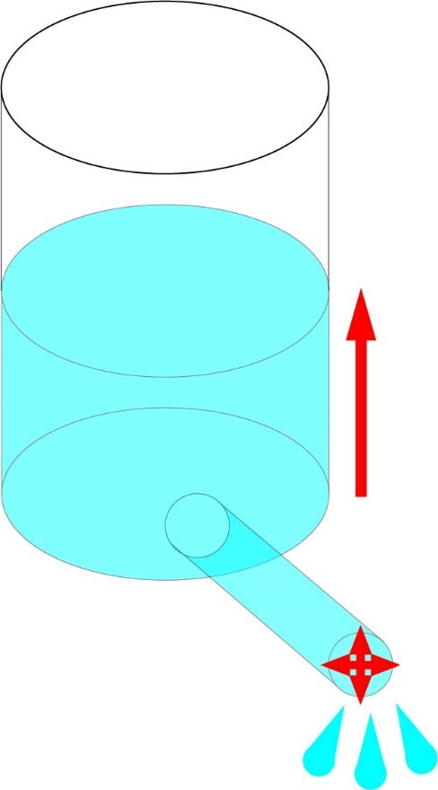
Fig 1. Either raising the water level (representing increased voltage) or increasing the diameter of the hose (representing decreased resistance) will increase the flow of water (representing current) out of the vessel.
This model would work well if all conductive materials had the same amount of resistance in relation to their volume and length, but that is not the case. Therefore a way to improve the model would be to think of the hose as filled with a porous material, such as finely packed sand or loosely packed cotton. This is a good way of thinking about it, since in a solid conductive material the charge carriers (electrons) flow through the matter around the nuclei, with the interactions between the charge carriers themselves and the nuclei causing resistance (called electron-phonon interactions). This is similar to the resistance that water sees flowing through a porous substance, where the resistance to flow is caused by the water itself (since water has volume) as well as the solid part of the material.
With the resistive material it becomes obvious that the longer the water has to travel through the resistive material the more restricted the flow will be, ie with a hose full of packed sand you can expect the flow to double if you cut the hose in half. So now we have three ways that we can reduce resistance; we can still increase the diameter of the hose, decrease the length of the hose, or use a more porous material inside the hose (see Fig. 2). In this case using a more porous material is equivalent to using an electrically conductive material with lower electrical resistivity.
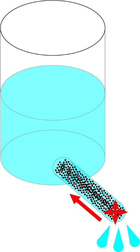
Fig 2. With a hose filled with a resistive material, such as porous stone or packed sand, flow can be increased by shortening the hose, increasing the diameter of the hose, or using a looser filling (representing using a material with reduced resistivity).
We can calculate the resistance of a piece of conductive material if we know its dimensions and its electrical resistivity, ρ, commonly measured in Ω·m or Ω·mm (ohm meters or ohm millimeters). ρ can vary significantly between materials; ρ of silver, the most conductive elemental metal, is 15.87 nΩ⋅m, whereas for pure silicon it is 2.3 kΩ⋅m, more than 11 orders of magnitude difference (I should point out that silicon electrodes are not pure silicon. Pure silicon is a semiconductor and would not provide a usable signal; instead it is doped to act as a conductor, although even doped silicon it is still significantly more resistive than metals). The relationship between resistance and resistivity is ![]() , where l is the length of the material and A is the cross sectional area (see Fig. 3).
, where l is the length of the material and A is the cross sectional area (see Fig. 3).
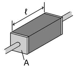
Fig 3. The resistance of an individual conductive element is a function of it’s resistivity, length, and cross-sectional area. Image from Wikipedia.
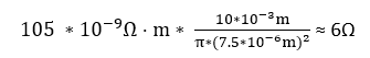
Let’s use this formula to calculate a sample impedance; let’s say for a 10mm long piece of cylindrical platinum wire, with a 15um diameter, insulated on the sides. Platinum is a metal commonly used for electrodes both for its stiffness (less likely to deform during implantation) and inertness (which increases its biocompatibility). Actually, platinum electrodes are usually a Platinum-Iridium alloy (pure platinum is much softer), but as an alloy the electrical properties can vary with alloy proportions, so for simplicity we’ll stick with pure platinum in this example, which as you’ll soon see won’t have a significant effect on the results. Platinum has an electrical resistivity of 105 nΩ⋅m, so a 10mm long platinum electrode with a diameter of 15μm (or radius of 7.5μm), insulated on the sides, would have a resistance of:
And this is what you would measure if you connected an ohm meter directly to the electrode. However that is not the way we measure impedance, not because it is difficult, but because the measurement wouldn’t be very useful. Instead we immerse the electrode in saline as this gives us results much closer to an electrode in tissue, and if you have ever measured the impedance of a platinum electrode (or just about electrode designed for electrophysiology) in saline or in vivo you have likely found that the impedance is many magnitudes of order higher; on the order of tens of kiloohms (1kΩ = 103Ω ) to megaohms (1MΩ = 106Ω). Obviously since the current has to pass through the saline to reach the electrode, the resistance of the saline will have an effect. However we know the resistivity of saline (although it varies with salinity, i.e. how much salt is dissolved in the water), and although it is many orders of magnitude higher than metal (about 3 *10-1m in salinities close to cerebrospinal fluid or CSF), the cross-sectional area is much larger (the diameter of your beaker is measured in cm rather than μm), so if we were to use the above formula to calculate the resistance of a beaker of saline it would also be on the order of ohms. Obviously something else is going on here, and what that is that whenever you put a solid conductor into an electrolyte, you get what is known as an electrolytic capacitor. Capacitance is one of the main components of reactive impedance (the other being inductance, however inductance has far less impact that capacitance in electrophysiological recordings so we will not discuss it in this article), so let’s examine capacitance and how it affects impedance.
What is capacitance?
The parallel plate capacitor
Capacitance is the ability of an object to store charge. It is measured in farads (F), named after Michael Faraday, whom the Faraday cage, another useful tool for electrophysiologists, is also named after. Capacitance is defined as C = q/V, where C is the capacitance, q is the charge, and V the potential or voltage. As you can see from the formula, at a fixed voltage, the larger the capacitor the larger the amount of charge it can hold. A one farad capacitor can hold one Coulomb of charge when allowed to fully charge from one volt. Although one volt is a small potential, one coulomb of charge is huge; allowed to quickly dissipate into a human body it would easily kill that person. One farad is also a huge amount of capacitance; usually the size of a large coffee can. You will not likely encounter a 1F capacitor outside of a power station, so the units μF, nF and pF are more commonly used (a picofarad is 10-12 farads). Since capacitors hold charge, and current is the flow of charge, and impedance is the resistance to flow of charge, it should be easy to see that capacitance will have a large effect on impedance.
The simplest form of a capacitor is a parallel plate capacitor; as the name implies it is made up of two parallel plates of conductive material with a dielectric in between. It is the inspiration for the schematic diagram symbol of a capacitor. A dielectric is an insulating material, ideally with high permittivity, i.e. it will not pass current but polarize more strongly in an electric field, allowing more charge to be held at either end (see Fig. 4). The capacitance of a parallel plate can be calculated using the formula C = εA/d, where ε is the permittivity of the dielectric, A is the area of the parallel plates, and d is the distance between the plates or thickness of the dielectric (see Fig. 5).
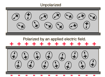
Fig 4. A material with higher permittivity is more easily polarized in an electric field, and able to hold more charge at its surface. Image from Wikipedia.

Fig 5. Structure of a parallel plate capacitor. Image from Wikipedia.
If a battery is connected to a capacitor (see Fig. 6), electrons will flow out of the negative terminal of the battery and start charging what is now the negative plate of the capacitor. Likewise electrons will flow from the positive plate into the positive terminal of the battery, both pulled by the positive charge of the positive terminal, and repelled by the negative charge building up on the negative plate. This will continue until the capacitor has the same voltage as the battery, at which point the capacitor is fully charged with a charge of q = CV and the current will stop. How long this takes is determined by both the size of the capacitor in farads, and the resistance of the entire system, or circuit (the battery, wires and capacitor itself will all have some small amount of resistance), so that τ = RC, where τ, called the time constant, is the amount of time it will take to charge the capacitor to about 63.2% of its capacity (63.2 ≈ 1-e-1). Likewise if the charged capacitor is then detached from the battery and attached to a new circuit of resistance Rn, τn will be the amount of time for the capacitor to discharge to about 36.8% of its capacity (36.8% ≈ e-1). Charging can be modeled as V(t) = Vo(1-e-t/τ) where V(t) is the voltage across the capacitor at any given time, and Vo is the initial voltage (zero if uncharged). Likewise discharging can be modeled as V(t) = Vo(e-t/τ). This time constant will have some interesting consequences when we start looking at what happens when we put an alternating voltage across the voltage.

Fig 6. If a battery is connected to capacitor, the positive side (cathode) side of the battery will pull electrons from the side of the capacitor it is connected to, while the negative side (anode) will push electrons to the opposite side. This will create a growing voltage potential across the capacitor that will climb toward the battery voltage. A larger capacitor will take longer to reach this maximum charge, but will ultimately hold a larger charge.
If we put a sinusoidally alternating voltage across the capacitor, the voltage source will alternate between which plate it is pushing charge into and which it is pulling it from. However, whichever plate is being charged will be at a point of maximum charge when the sinusoid transitions, i.e. the sinusoid is at 0V between the positive and negative phase or vice versa (see Fig. 7), after which the voltage flips polarity and charge is moved to the opposite plate. Since that is the point of maximum charge, it is also the point of maximum repulsion from the charge on the negative plate. As a result, while a capacitor will stop current from flowing once it is charged from a direct voltage (at that point act as an open circuit, or infinitely resistive), an alternating voltage will pass indefinitely, but will be phase shifted by some amount less than 90֯ (it would be exactly 90֯ if there were no resistance, but since that is physically impossible it will be some amount less; this will be equal to the phase of the complex impedance as we will describe shortly).

Fig 7. Phase shift created by a capacitor. With a sinusoidal input, the point of maximum charge on the leading plate will create maximum repulsion. If the resistance of the circuit were zero this would be the point of maximum inverted voltage, creating a phase shift of exactly -90⁰. Greater impedance will reduce the magnitude of this phase-shift
Using the hydraulic model we can more intuitively understand a capacitor as a flexible membrane across the inside of a sealed tube of water. Exerting a constant pressure of water on the membrane will cause it to stretch; the greater the pressure the greater the membrane will stretch and the greater the volume of water the stretched cavity will hold (equivalent to the amount of charge). A more flexible membrane (higher capacitance) will stretch further at the same amount of pressure, but regardless will eventually stop the flow of water. If the pressure is removed, the membrane will spring back and create a flow of water in the opposite direction, just as a capacitor will relinquish its stored energy by giving back the charge it held, creating a current opposite to the current that charged it. If you were to apply an alternating pressure, a stiffer membrane (lower capacitance) will translate less of the alternating pressure to the other side, creating more resistance to the movement of water. Electrical capacitors work the same way, and their impedance at a given frequency is inversely proportional to their capacitance. Just as a capacitor is an open circuit to a direct voltage, its impedance also drops off with higher frequency. The impedance of a capacitor can be calculated as ![]() , where C is the capacitance and 𝑓 is the frequency of the driving voltage or current. Notice that impedance is commonly denoted as a “Z” to indicate that it is a complex number, including both real (resistance) and imaginary (reactance) components. The j is to indicate that it is an imaginary number equal to √(-1) (mathematicians more intuitively use i for imaginary numbers, but engineers generally use j to avoid confusion with current). Complex numbers are a topic that are too complex for the scope of this article (although Wikipedia has an excellent explanation), it is enough for our purposes to know that normal numbers are scalars, having only magnitude, whereas complex numbers are vectors, having both magnitude and direction, or phase. The magnitude of a complex number can be calculated using Pythagorean’s theorem, and the phase with trigonomic functions (i.e. for a 1Ω resistor in series with a 1F capacitor driven by alternating voltage with a frequency of 1/2πHz to give -1Ω of reactance, the magnitude of the impedance would be √(2), resulting in a current of (1/√(2))A phase shifted 45֯ relative to the voltage). Therefore, an impedance containing reactance will not only attenuate a signal, like a purely resistive impedance will, but also cause a phase shift. This will cause some interesting effects on a complex signal that is made up of more than simple sinusoids, as we will see later.
, where C is the capacitance and 𝑓 is the frequency of the driving voltage or current. Notice that impedance is commonly denoted as a “Z” to indicate that it is a complex number, including both real (resistance) and imaginary (reactance) components. The j is to indicate that it is an imaginary number equal to √(-1) (mathematicians more intuitively use i for imaginary numbers, but engineers generally use j to avoid confusion with current). Complex numbers are a topic that are too complex for the scope of this article (although Wikipedia has an excellent explanation), it is enough for our purposes to know that normal numbers are scalars, having only magnitude, whereas complex numbers are vectors, having both magnitude and direction, or phase. The magnitude of a complex number can be calculated using Pythagorean’s theorem, and the phase with trigonomic functions (i.e. for a 1Ω resistor in series with a 1F capacitor driven by alternating voltage with a frequency of 1/2πHz to give -1Ω of reactance, the magnitude of the impedance would be √(2), resulting in a current of (1/√(2))A phase shifted 45֯ relative to the voltage). Therefore, an impedance containing reactance will not only attenuate a signal, like a purely resistive impedance will, but also cause a phase shift. This will cause some interesting effects on a complex signal that is made up of more than simple sinusoids, as we will see later.
The electrolytic capacitor
So now let’s look at why a solid conductor in electrolyte acts as a conductor. You may be surprised to learn this, but pure water is actually an insulator. When two hydrogen atoms bind to oxygen, the electrons will sit deep in the electrostatic well of the oxygen nucleus. This creates a highly polar atom, with a strong positive charge on the side of the molecule with the hydrogen nuclei (protons), and a strong negative charge on the side with the oxygen nucleus. Because of this high level of electronegativity electrons cannot flow across the molecule, but it also makes water a very strong polar solvent, capable of dissolving compounds such as salts since it will rip positive and negative ions away from each other (it is because of this strong electronegativity that water is liquid instead of a gas at standard temperature and pressure, despite being made up of such light-weight molecules). With water full of anions (negative ions) and cations (positive ions), the ions can now freely flow, moving charge, and making water conductive. This is why you wouldn’t want to jump into a vat of purified water holding a plugged-in toaster; although initially the water wouldn’t conduct, the salts on the surface of your skin would immediately dissolve and the water would now have charge carriers available to give you a strong jolt. The more ions dissolved in the water the more conductive it is, so dissolving sodium chloride in water to match the molarity of dissolved ions in cerebrospinal fluid or the interstitial fluid of the brain and nerves will make a good model fluid to test the impedance of your electrodes.
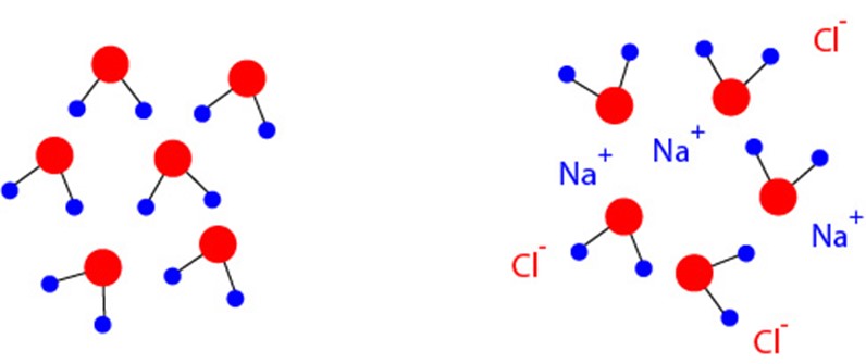
Fig 8. In pure water, represented on the left, all of the electrons are held by the potential well of the oxygen atoms (red circles), leaving the hydrogen nuclei as “exposed” protons (blue circles). This creates a strong electrostatic differential across each molecule, and there are no charge carriers to conduct current. If a salt (such as sodium chloride to make saline) is introduced to water these electrostatic gradients will pull the salts apart into cations and anions, creating free charge carriers that can move through solution to create electrical currents, as represented on the right.
The action potentials created by excited neurons are the result of the neuron controlling the flow of ions through ion channels, particularly sodium and potassium, but also calcium, chlorine, magnesium, etc. These ions can travel freely in solution, but cannot travel through a solid conductor. If a potential is created it will cause anions or cations to travel to the surface of the electrode, but they cannot penetrate the electrode to create a current the way that electrons can flow through solid conductors. Instead a flow of anions like chlorine toward the surface of the electrode will repel electrons away from the surface of the electrode, just the way that a flow of electrons into one plate of a parallel plate capacitor will cause electrons to be driven away from the plate/dielectric junction at the opposite plate. Similarly cations like potassium and sodium flowing towards an electrode will attract electrons to the surface of the electrode, just like a positive charge on one plate of a parallel plate capacitor drains it of electrons, creating a net positive charge that attracts electrons towards the opposite plate/dielectric junction (Fig. 9). It is these flows of charge carriers that can move freely within their medium, but not cross the solid conductor/electrolyte junction that creates a capacitive effect.

Fig 9. On the left, an electrode is in saline with an electrical potential driving the sodium ions towards the electrode/saline junction. This attracts the electrons towards the junction, creating a positive current flowing into the electrode. On the right the potential is reversed, and chlorine ions are driven to the junction. This repels the electrons in the electrode away from the junction, creating a net positive charge on the electrode side of the junction, and a positive current flowing out of the electrode.
Industrial electrolytic capacitors will oxidize the surface of the metal before placing it in electrolyte; this creates an easily definable dielectric layer that makes the capacitance easy to calculate, and therefore easy to design the dimensions needed for a specific capacitance value. Since an electrode in electrolyte does not have this clearly defined layer, capacitance is not easily predicted or calculated, however the capacitance of platinum in saline has been experimentally measured to be approximately 0.2pF/μm2 (DA Robinson, The Electrical Properties of Metal Microelectrodes. Proceedings of the IEEE, Vol 56, No 6, June 1968). If we use this value for our 15um diameter platinum electrode that we looked at earlier in the article, and a frequency of 1kHz (we will explain in the next section why we are using 1kHz), this a capacitance of ![]() , which gives us a magnitude of impedance of
, which gives us a magnitude of impedance of ![]() . Although this is actually about two orders of magnitude above what you would measure from a 15μm diameter platinum wire, we can see we are now getting into the ballpark. There are a few reasons for the difference (all of which are discussed in the Robinson paper if you would like more details), but the most significant is that an electrolytic capacitor actually has a leakage resistance in parallel with the capacitive load (see Fig 10, we will discuss later what loads in parallel and in series means, but for now know that any number of loads in parallel always have less total impedance than any individual load). This leakage resistance is created because cations and anions in solution can accept or give up electrons, and in turn transfer them to or from the solid conductor, creating a leakage current, hence the name.
. Although this is actually about two orders of magnitude above what you would measure from a 15μm diameter platinum wire, we can see we are now getting into the ballpark. There are a few reasons for the difference (all of which are discussed in the Robinson paper if you would like more details), but the most significant is that an electrolytic capacitor actually has a leakage resistance in parallel with the capacitive load (see Fig 10, we will discuss later what loads in parallel and in series means, but for now know that any number of loads in parallel always have less total impedance than any individual load). This leakage resistance is created because cations and anions in solution can accept or give up electrons, and in turn transfer them to or from the solid conductor, creating a leakage current, hence the name.

Fig 10. Equivalent circuit model of an electrolytic capacitor. Note that while the resistors noted represent simple resistance, they are being represented by the symbol more commonly used for a complex load consisting of resistance and reactance (ie a rectangle instead of a squiggle). This is to denote that these values are frequency-dependent. The symbol for LESL denotes inductance, which as previously mentioned is not explored in this article, and does not significantly contribute to the total impedance in the frequency ranges of interest to the electrophysiologist. Figure from Wikipedia.
We won’t repeat this calculation for a silicon electrode as there are too many variables (the level of doping will significantly affect all the values discussed), but the higher resistivity of the material will result in a lower capacitive value along with a lower leakage current, resulting in much higher total impedance. In general silicon electrodes have an impedance of around two orders of magnitude higher than a metal electrode with the same site diameter recording sites. However these values can also be changed significantly by doing things such as abrasive treatment of the electrode sites (this increases the surface area without increasing diameter, which in turn increases capacitance and leakage current, reducing impedance), or coating the recording sites with different conductive materials such as platinum black or PEDOT, which will also significantly affect capacitance and resistance, and therefore impedance.
Complex signals and frequency
So far we’ve been calculating our impedances in relation to a pure sinusoid voltage of 1kHz; this (or a frequencies close to it) is the default frequency generally used by most impedance measurement devices (such as the nanoZ or IMP, although they are capable of measuring at different frequencies) and by electrophysiologist in general. Let’s take a look at why that is.
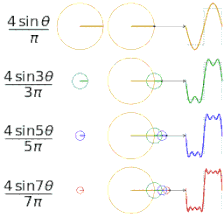
Any biological signal is unlikely to be a pure sinusoid, however any signal can be constructed by summing up an infinite series of sinusoids, known as a Fourier series (as illustrated below in Fig. 11). Likewise a Fourier transformation can be performed on a signal or function to show the power spectrum of a signal, ie where the energy of the signal lies in relationship to frequency (see Fig. 12). If you were to perform a Fourier transformation on a signal, then use that spectrum to calculate the effects of your complex impedance, by transforming those results back into the time-amplitude domain (ie perform an inverse Fourier transformation), you can calculate how any signal would be affected by a complex impedance. The mathematics of a Fourier series and Fourier transform are beyond the scope of this article (although if you’d like to learn more, the wikipedia pages are very informative, or you could look at just about any textbook on signal processing), but having an awareness of these concepts will help understand why frequency is important to electrophysiology.
|
Fig 11. A square wave being approximated by the sum of the first four terms of its Fourier series. Animation from Wikipedia. |
Fig 12. The relation of a signal, its Fourier series (using the first 6 terms), and its Fourier transform/power spectrum. Animation from Wikipedia |
In this article we will use the Fast Fourier Transform (called FFT for short) on various signals to illustrate the effects of frequency. The FFT is an approximation of the Fourier transformation that can be done on a digitized signal with a digital processer. Fig. 13 shows a 1V, 10Hz sinusoid plotted in the time domain on the top, and frequency domain on the bottom using an FFT calculated in MATLAB. A Fourier transform would simply be a vertical line at 10Hz, with an amplitude of 1, and zero elsewhere, but the FFT approximation is more than close enough to be useful for our purposes. Likewise Fig. 14 shows approximated white noise (generated using MATLAB’s rand function). A Fourier transformation of true white noise would be a horizontal line. The FFT shows the limitations both of an FFT of a limited sample size and in digitized signals; it is limited in the higher frequencies to half the sampling rate (called the Nyquist frequency), and the power isn’t accurately measured in the lower frequencies due to the short length of time of the signal. In both cases the FFT would more closely resemble the results of a Fourier transform with a larger sample set (either by sampling at a higher frequency, or recording the signal for longer).
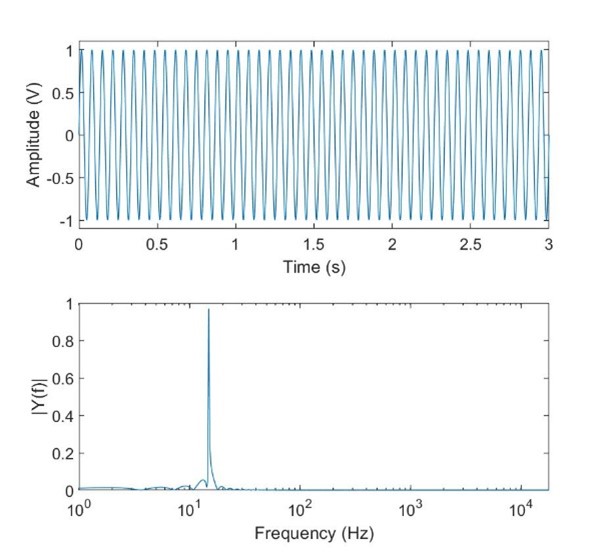
Fig 13. A 10Hz sinusoid plotted in the time and frequency domains.
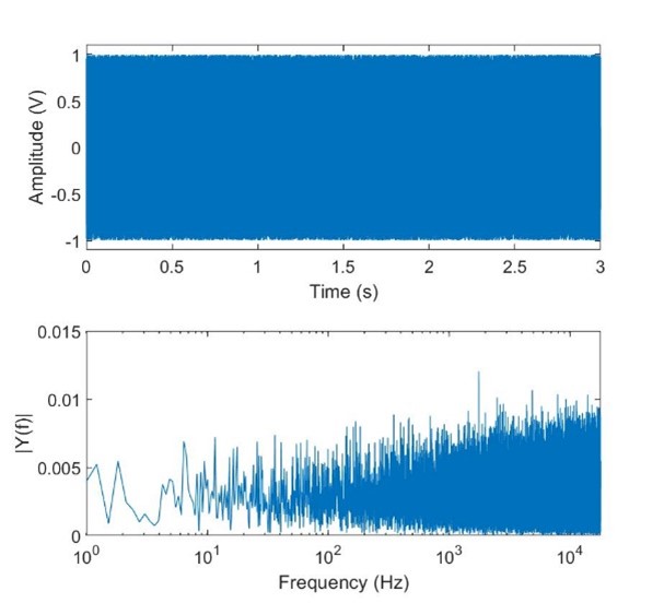
Fig 14. Approximated white noise.
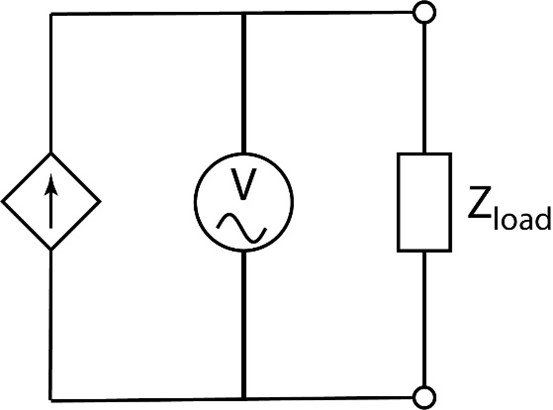
Let’s now take a look at how an impedance meter works. Basically an impedance meter is a current source that feeds a current of known frequency and amplitude into a test load (in our case an electrode in saline, or for an in vivo test, and electrode inserted into a subject), and then records the resulting voltage across the test load (see Fig 15.). Using Ohm’s law for a complex impedance, Vload = Itest x Zload, we can measure the magnitude of the impedance of that load by comparing the amplitudes. By comparing the phase difference between the test current and resulting voltage, we can also calculate how much of the impedance is real (resistance) and how much is imaginary (reactance), and therefore measure the simple resistance and capacitance of the electrode. Pure sinusoids are used because they are easy to accurately produce with an oscillating circuit, easily measured, and since the mathematics are simpler, easier to accurately assess the results digitally. By varying the frequency of the test signal used, we can measure the impedance spectroscopy of the electrode, which is a curve of impedance vs. frequency (see Fig. 16 for an example impedance curve of an S-probe measured with the impedance spectroscopy feature of a nanoZ). If we know the frequency characteristics of the signal of interest, we can then use the impedance curve to predict how the electrode impedance characteristics will impact our recordings.
|
Fig 15. Simplified schematic of an impedance tester. A controllable AC current source of variable frequency is fed into the load impedance (the electrode in saline or in vivo), and a voltameter measures both the amplitude and phase of the voltage across the load. This allows both the resistance and reactance to be calculated. |
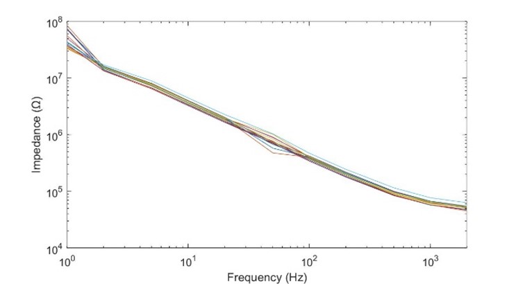
Fig 16. Impedance spectograph of a 16 channel S-probe with 15μm diameter recording sites. Recorded with a nanoZ from 1.005Hz to 2kHz. Both axes are logarithmically scaled. Notice that the impedance drops from tens of megaohms in the hertz range to tens of kilohms in the kilohertz range. |
Since we are interested in recording single units, let’s take a look at an action potential. Fig. 17 shows a pile plot of several action potentials from a single unit recorded on an Omniplex system, from an anesthetized mouse acutely implanted with a Michigan array. The units were thresholded and separated in Offline Sorter, and one unit selected and exported to Matlab for analysis. Overlaid on the pile plot is one cycle of a 1kHz sinusoid for comparison, with the peak of the cycle time-aligned with the peaks of the action potentials. As you can see from the comparison, the main body of the action potentials are a little bit thinner than the cycle of the sinusoid, suggesting a center energy that’s a little higher than 1kHz. And indeed, if we look at the FFT we can see that the peak energy is close to, but a little higher than 1kHz. This will vary a little bit among different neurons and types of neuronal populations, however we can see that this is why we measure impedance at 1kHz (or near 1kHz), since that is the lion’s share of where the energy lies in single units, and where the signal will be impacted the most.
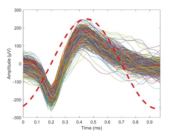
Fig 17. A pile plot of action potentials recorded from a single unit with a 1kHz sinusoid overlaid for comparison

Fig 18. FFT of the action potentials
This of course assumes that your focus is single units. If you are more interested in local field potentials or electrocorticography, then you will want to pay more attention to the lower end of the frequency spectrum. However, we will soon see that there are several factors that make recording these signals much less challenging, and therefore do not usually require the same level of attention.
Resistance and capacitance in series or in parallel
Let’s briefly talk about loads in parallel and in series since they have an effect on measurement and noise. Figure 19 shows the schematic representation of loads in parallel and in series, and as you can see series means that the circuit elements are placed so that current through one element must pass through the other, while in parallel, the current is given two paths and so will be divided between the two elements.
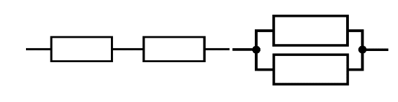
Fig 19. Schematic representation of impedances connected in series (left) and in parallel (right)
If two resistors, R1 and R2 are placed in series, the series resistance is simply the sum of the two resistors, RS = R1 + R2; if R1 and R2 are equal the impedance is doubled. This makes sense from our discussion of the architecture of a resistor (from Fig. 3, and our formula ![]() ), as if you made two identical resistive elements and put them end-to-end, you essentially one resistor twice as long, which would have double resistance. Using our hydraulic model, you can think of connecting two hoses of equal length full of dense sand end-to-end; the flow of water would be half as that running through a single hose.
), as if you made two identical resistive elements and put them end-to-end, you essentially one resistor twice as long, which would have double resistance. Using our hydraulic model, you can think of connecting two hoses of equal length full of dense sand end-to-end; the flow of water would be half as that running through a single hose.
If two resistors are placed in parallel, you are now giving the current two paths to flow through, which will allow for more current, so the resistance drops. The parallel resistance can be calculated as ![]() . If the resistors are equal this simplifies to R/2. This again makes sense using our formula for resistance, as if you were to put two identical resistive elements side-by-side, this would be the same as a single resistor with twice the cross-sectional area, and therefore the resistance would be half. Likewise in the hydraulic model, if you were to insert a second hose in your cylinder of water, you would expect to double the rate of flow of water out of it.
. If the resistors are equal this simplifies to R/2. This again makes sense using our formula for resistance, as if you were to put two identical resistive elements side-by-side, this would be the same as a single resistor with twice the cross-sectional area, and therefore the resistance would be half. Likewise in the hydraulic model, if you were to insert a second hose in your cylinder of water, you would expect to double the rate of flow of water out of it.
The relation for capacitors in series and parallel is reversed; two capacitors in parallel are the sum of the two capacitances, i.e. Cp = C1 + C2, and capacitors in series have reduced capacitance,  . Again we can see why this is if we look at the architecture of a simple capacitor (Fig. 5 and our formula
 ![]() two equal capacitors side-by-side would effectively be one capacitor with double the area, and therefore have double the capacitance. Likewise two equal capacitors in series would be the equivalent of a single capacitor with a dielectric twice as thick (so d is doubled), resulting in half the capacitance. In our hydraulic model, two capacitors in parallel is equivalent to a membrane with double the material (i.e. stretched half as much), making it more stretchy and able to hold more water at the same pressure. Two capacitors in series would be like a doubled membrane, or one twice as thick and therefore twice as stiff, making it stretch less at the same pressure.
two equal capacitors side-by-side would effectively be one capacitor with double the area, and therefore have double the capacitance. Likewise two equal capacitors in series would be the equivalent of a single capacitor with a dielectric twice as thick (so d is doubled), resulting in half the capacitance. In our hydraulic model, two capacitors in parallel is equivalent to a membrane with double the material (i.e. stretched half as much), making it more stretchy and able to hold more water at the same pressure. Two capacitors in series would be like a doubled membrane, or one twice as thick and therefore twice as stiff, making it stretch less at the same pressure.
For complex loads containing resistance and reactance, the same relationship applies as for resistance, i.e. ZS = Z1 + Z2 and ![]() , however you would use complex numbers for the reactance. Since the reactance for a capacitor is
, however you would use complex numbers for the reactance. Since the reactance for a capacitor is ![]() , we can see that in the cases of purely capacitive loads, we get the same results when calculating series or parallel resistances regardless if we calculate the equivalent capacitance first, and use that to calculate the impedance, or if calculate the impedances directly. For instance, two equal capacitors in series would have half the capacitance, therefore plugging in the equivalent capacitance gives you
, we can see that in the cases of purely capacitive loads, we get the same results when calculating series or parallel resistances regardless if we calculate the equivalent capacitance first, and use that to calculate the impedance, or if calculate the impedances directly. For instance, two equal capacitors in series would have half the capacitance, therefore plugging in the equivalent capacitance gives you ![]() , which is the same as
, which is the same as ![]() , the result you get from summing the reactive impedances.
, the result you get from summing the reactive impedances.
Noise (ie electrical signals not related to the signal we are trying to acquire) arises in the subject, the amplifier we are using to record the signal, and to a lesser degree even the electrode itself (mostly thermal noise and a small amount of EMI; in most cases this is almost negligible so for simplicities sake we won’t include it in the model below. However, this is a gross simplification, and in particular thermal noise in a high impedance electrode will be a significant part of the noise floor; for more detail I recommend The Noise and Impedance of Microelectrodes, Michael Mierzejewski et al 2020 J. Neural Eng. 17 052001). For a description of sources of noise and strategies to mitigate them, see my previous blog “Causes of Noise in Electrophysiological Recordings” which can be found here.
Fig. 20 shows an equivalent circuit of an in vivo electrode connected to an amplifier. The amplifiers used in electrophysiology are voltage amplifiers; that is they read the voltage at their inputs, add gain, and output a voltage (an example of a different type of amplifier is one generally used for electrical stimulation, which is a transconductance amplifier; ie it reads the voltage at its inputs, and outputs a current proportional to the input voltage, which we will discuss in the section on microstimulation. It is so named because the gain is measured as Iout/Vin. We recall from Ohm’s law the resistance is voltage divided by current, so current divided by voltage is the inverse of resistance, which is conductance. Current amplifiers and transresistance amplifiers also exist). Amplifiers have an input impedance, and ideally a voltage amplifier will have an input impedance as high as possible to reduce the effects of any impedance between the amplifier and signal source (which our case is dominated by the electrode impedance).
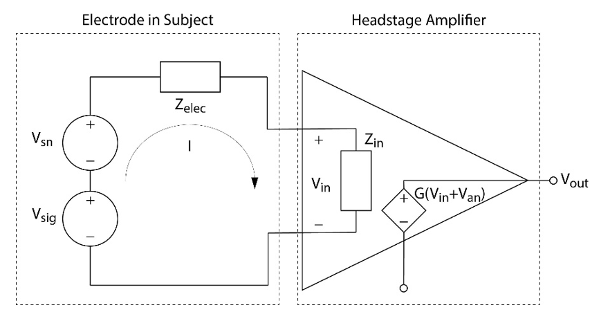
Fig 20. Electrical schematic representation of an electrode implanted into a subject and connected to a headstage amplifier. The noise present in the subject (Vsn) is added to the electrophysiological signal (Vsig), and together they create a current I that runs through both the electrode (Zelec) and input of the amplifier (Zin). This creates a reduced voltage at the amplifier’s input, which is amplified along with the noise of the amplifier (Van).
From Fig. 20 we can see the potential we are recording is driving against the impedance of the electrode along with the input impedance of the amplifier in series. This will create a current through both loads where ![]() . However, it is the voltage at the input of the amplifier that is being amplified, which is equal to I*Zin, therefore
. However, it is the voltage at the input of the amplifier that is being amplified, which is equal to I*Zin, therefore ![]() . When the impedance of the electrode is much less than the amplifier’s input impedance, Vin relative to the signal and subject noise is mostly unaffected, but starts to become significantly attenuated as the electrode impedance approaches, or even surpasses the input impedance of the amplifier.
. When the impedance of the electrode is much less than the amplifier’s input impedance, Vin relative to the signal and subject noise is mostly unaffected, but starts to become significantly attenuated as the electrode impedance approaches, or even surpasses the input impedance of the amplifier.
However, this will affect the electrophysiological signal and subject noise equally, and since what we need to capture our spikes is a good signal-to-noise ratio (SNR), which is the signal divided by the noise (see Fig 20), at first glance it would seem that electrode impedance has no relation to SNR, but that is before we take into account the noise of the amplifier that is added to the signal before it is amplified, and so is always present regardless of the amplitude of the signal; Vout = G(Vin + Van). The gain, G, is generally optimized to give the best results when connected to the digitizer, which in turn will generally scale down the signal so that the system is reporting the true amplitude of the signal.
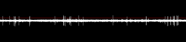
Fig 20. A strong signal-to-noise ratio allows for spikes to stand out clearly for thresholding and accurate sorting. Image taken from the timeline view of Offline Sorter after high-pass filtering wideband data.
Let’s use some real-world values to get an idea of how impedance impacts SNR in practice. Currently the most commonly used amplifier for electrophysiology is by far the Intan RHD2000 family of chips. Prior to the Intan chip, a small, analog buffering headstage would be used, that would then be sent to a larger amplifier and then digitized to be sent to the main chassis for processing. The buffering headstage was used to make the signal less subject to noise (the amplitude of an unbuffered units is insignificant to the amount of EMI picked up by a headstage cable), but it was still an analog signal and subject to both EMI and movement artifacts caused by movement in the cable. The Intan chip miniaturized all of the amplification and digitization circuitry into a single IC chip, allowing all of the signal conditioning and digitization to occur on the headstage. Once the signal is digitized, it is immune to noise (except in the extreme case that it is so large the 0 and 1 bits can’t be distinguished, in which case you lose communication with the headstage and you stop receiving a signal altogether). All of the major multichannel electrophysiological system providers use Intan chips for their digitizing headstages, including Plexon.
Looking at the Intan RHD2000 datasheet (link in the references section), we can see that the input inferred noise of 2.4μVrms (input inferred noise is the output of the noise of the amplifier divided by its gain, so this noise will be amplified equally with the recorded signal and recorded noise, and so is effectively the lowest possible noise floor for the amplifier that we can get) and an input impedance of 13MΩ at 1kHz. Let’s say we have a single unit producing action potentials with an amplitude of 50μVpk, in an environment where we’ve diligently shielded or removed noise sources, and have a very low noise in the subject of 2.50μVpk(for simplicity we are ignoring noise originating in the electrode). We can convert Vrms to Vpk by multiplying by 2, which gives us a value of ~3.4μV peak (another simplification; SNR is usually recorded using the ratios of the power of the signals involved instead of the peaks; RMS, or root-mean square is useful for this, but for simplicity we are going to use peak values since it requires less math and is easier to visualize). If we were to record from the signal using a 1MΩ electrode, the drop in amplitude for the action potentials and subject noise as seen by the amplifier will be fairly small, ![]() ≈ 93% of the original values, or a spike amplitude 46.4μV and a subject noise of 2.32μV. Plugging these values gives us an SNR of our spikes to noise floor to be
≈ 93% of the original values, or a spike amplitude 46.4μV and a subject noise of 2.32μV. Plugging these values gives us an SNR of our spikes to noise floor to be ![]() ≈ 16:1. With such a high ratio, it will be easy to threshold our spikes. Now let’s look instead at recording with a 100MΩ electrode. The drop in amplitude of the spikes and subject noise will now be very significant,
≈ 16:1. With such a high ratio, it will be easy to threshold our spikes. Now let’s look instead at recording with a 100MΩ electrode. The drop in amplitude of the spikes and subject noise will now be very significant, ![]() ≈ 11.5% of the original values, or a spike amplitude 5.75μV and a subject noise of 0.288μV. Plugging these values gives us an SNR of our spikes to noise floor to be
≈ 11.5% of the original values, or a spike amplitude 5.75μV and a subject noise of 0.288μV. Plugging these values gives us an SNR of our spikes to noise floor to be ![]() ≈ 1.6:1. The spikes will now be just peeking out over the noise floor, and the waveforms themselves may be too distorted to use for spike sorting, as most of the samples will be in the noise floor. And this is under best conditions with a number of simplifications that actually significantly understate the effect; in practice a 100MΩ electrode will generally give you an SNR of less than one; ie the spike will be completely buried in noise. This is why commercial manufacturers of microarrays will use designs that provide impedances of approximately a couple megaohms at most unless they are designed to be used with particular amplifiers with very high input impedance.
≈ 1.6:1. The spikes will now be just peeking out over the noise floor, and the waveforms themselves may be too distorted to use for spike sorting, as most of the samples will be in the noise floor. And this is under best conditions with a number of simplifications that actually significantly understate the effect; in practice a 100MΩ electrode will generally give you an SNR of less than one; ie the spike will be completely buried in noise. This is why commercial manufacturers of microarrays will use designs that provide impedances of approximately a couple megaohms at most unless they are designed to be used with particular amplifiers with very high input impedance.
From the examples above we see that SNR drops rapidly as we approach the input impedance of the amplifier, but even at values far smaller, impedance does negatively impact SNR. Since electrodes can be made with much smaller impedances (for example, ECoG electrodes are usually in the range of a kiloohm), why do we bother with high impedance electrodes at all? The answer to that will be explored in the next section.
Causes of Noise in Electrophysiological Recordings, Plexon blog post June 28th, 2021
There are two major factors that determine how well a unit is isolated, the distance of the electrode site from a neuron, and the size of the electrode site relative to the neuron. As shown in Fig. 22a, an electrode site with a diameter that is on the order of or smaller than the diameter of the soma of a target neuron, and in very close proximity will be dominated by the electrical activity of that neuron, giving excellent isolation that can rival that of an intercellular electrode. It will also still be possible to filter the signal for local field potentials, although the “reach” of the local field potentials will be less than that of larger diameter electrode, ie the local field potential signal will be more localized. If the electrode site is in the range of up to roughly an order of magnitude larger than the target cells (Fig. 22b), then you are more likely to see a summation of a small number of local cells, ie multi-unit activity. This is a sacrifice in signal quality compared to a single unit activity, however it allows you to reliably identify multiple cells from a single recording site, with significantly reduced impedance (and therefore a lower noise floor), and greater longevity for long-term chronic recordings (we’ll visit why shortly). Electrodes with recording sites much larger than the size of individual cells won’t be able to resolve single units at all, but can record from larger areas of cortex, making them ideally suited for recording field potentials from larger areas, without the impedance and longevity issues of smaller recording sites. This is what FP, EEG and ECoG electrodes are targeting (Fig. 22c).
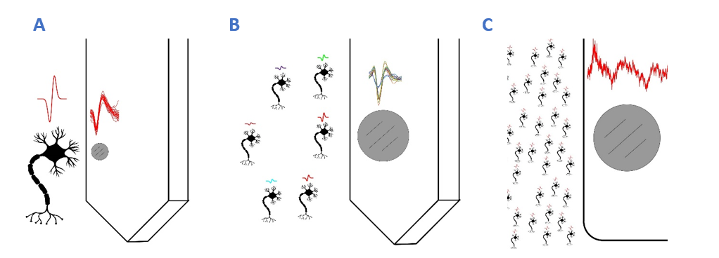
Fig 22. Unit isolation is determined by electrode size and proximity to the target neurons. A) If the electrode site is close to a neuron, and is about the same size or smaller, it will be dominated by the activity of that neuron. The signal can be filtered for field potentials, but the range will be very localized. B) If the electrode site is larger than a neuron, but on a similar scale, multiple units can be recorded on a single electrode, and filtered field potentials will cover a larger area. C) Electrodes orders of magnitude larger than a neuron will not be able to resolve single units but can see the sum of activity over a large area of cortex.
The sizes of different neuron populations can vary significantly depending on the type of neuron, from roughly 5μm in diameter (ie granular cells in cerebellum) to about 100μm (ie giant pyramidal cells in motor cortex). Knowing the anatomy of your target population can help you optimize your recordings, but in general electrodes for single-unit activity should have recording sites with 15μm or less in diameter, multi-unit electrodes are generally in the range of 30-60μm in diameter, and FP, EEG and ECoG electrodes are generally 250μm to 2mm in diameter.
As we’ve seen, unit isolation is a function of electrode diameter, and diameter is directly related to impedance, but since impedance is also determined by electrode material, and can be significantly altered using site coatings or treatments, using electrode impedance to predict single unit quality is only useful when comparing electrodes of the same material and design.
As mentioned previously metal electrodes will have an impedance of roughly two orders of magnitude less than silicon electrodes with the same diameter sites. Since we know that higher impedance means higher noise, why do we use silicon electrodes? There are two reasons; the first is for their stiffness, and the second and more significant reason is that by using silicon we can take advantage of the microfabrication techniques that have been developed over the last several decades with trillions of dollars of investment from the semiconductor industry.
Regarding stiffness, metals are malleable, so if presented with even a small force, they will deform, even if to a small degree. Since silicon is rigid, it will not deform until it breaks. That is something of a double-edged sword, since that means that silicon electrodes are extremely fragile and need to be handled with the utmost care to avoid fracturing them, but on the upside if your silicon electrode array is implanted and you are getting good signals from it, you can be certain the array geometry is intact. Since metal is malleable, electrodes from metal are either made to be much thicker than the electrode site (electrode sites much smaller than the thickness of the wire can be reliably made by insulating the wire and then using a fine laser to ablate the insulation), or it has to be laid upon a thicker substrate to get enough stiffness for it to be able to survive implantation without excessive deformation; this limits how densely metal microelectrode arrays can be spaced. While modern fabrication techniques have produced metal-based arrays with 32 or more channels that can fit in subjects as small as a mouse, they cannot compare to the density that silicon arrays can now achieve, such as the NeuroPixel and SiNAPS probes that can fit hundreds to more than a thousand channels on a single shank less than a couple hundred micrometers wide. It is because of these contrasting limitations and advantages that you never see single electrodes made of silicon, or silicon electrodes with a recording site diameter of less than about 10 μm. Likewise, barring any sudden leaps in fabrication technology, you are not going to see metal electrodes with densities anywhere near the densest silicon arrays any time soon.
Fig 23. Taking advantage of modern semiconductor fabrication techniques allows for microelectrode arrays of extreme density. Shown is a single-shank SiNAPS probe only 120μm wide with 256 recording sites.
Changes to the Impedance of Electrodes Over Time
Both implanted electrodes and acute electrodes that are reused are subject to a number of effects that will affect both their longevity and their impedance over time. A solid conductor in electrolyte can exchange ions and undergo chemical reactions such as oxidation that change the electrical properties over time, resulting in increasing impedance; this effect can be reduced by coating the electrode sites with more inert materials. Being a foreign body, the electrodes will be targeted by the body’s immune response and over time will be coated with platelets; smaller electrodes sites will be much more strongly impacted by this since they are more easily occluded. For electrodes that are reused, biological material will cling to the electrode sites and can dry out if not cleaned off immediately, forming a resistive layer that can be very difficult to remove.
For these reasons it is always a good idea to measure the impedance of an electrode before implantation, periodically during chronic recordings, after retrieval if the electrode is going to be reused, and before storage if the electrode is going to be stored for a long time.
Measuring the impedance prior to implantation prevents wasting time and potentially a subject by implanting a damaged electrode and provides a baseline measurement to compare against. This can be helpful during implantation (as electrodes suddenly reading much higher impedances can indicate poor placement or damage during implantation), and for assessing the condition of the electrode over time. Getting in the habit of periodically testing impedance in vivo in an implanted electrode will help with developing surgical technique (as you’ll be able to identify which surgeries led to longer usable implantations) and troubleshooting techniques. If using a chronic microdrive it can also help you know when you will benefit from moving the electrode. Measuring elevated impedance after retrieval and cleaning can be a strong indicator if there is any biological material remaining on the recording sites; removing it before it gets a chance to dry and harden will increase the longevity of the probe (for the same reason it is also good to test impedance before storing a probe). Large changes in impedance can also be an indicator that the electrode would benefit from recoating or rejuvenating the electrode sites.
Unfortunately, successfully microstimulating can be more complicated than simply connecting a stimulator and dialing in the desired current. Unexpected results can range from simply not inducing the expected effect, to killing the subject. In this section we will explore some of the more common reasons that lead to unsuccessful stimulation.
Compliance voltage
As mentioned previously, most cortical stimulators are transconductance amplifiers; ie they are controlled with an input voltage and output a current proportional to the input voltage. As we have seen how much impedance can vary with frequency and different electrodes, this produces results that are far more easily controlled than by trying to stimulate with a voltage source. However, despite being current sources, cortical stimulators are limited both in the total voltage and current that they can output (as is true with all amplifiers). From ohm’s law, we know that the current driven through the electrode will produce a voltage equal to the stimulation current times the in vivo impedance of the electrode; this voltage cannot exceed the compliance voltage of the stimulator, which is the limiting voltage of the stimulator. This voltage is always less than voltage used to power the output stage of the stimulator (due to some voltage loss in the circuitry); if this limitation didn’t exist the amplifier would be outputting more power than it consumes, which would violate the law of conservation of energy, so it is impossible to design an amplifier without a compliance voltage. Most commercial stimulators have a compliance voltage of about 8-12 volts, although some clinical stimulators can have compliance voltages of more than 100 volts (although care should be taken when using such a stimulator, since such a high compliance voltage can create dangerous conditions that can easily damage tissue, as we will soon see). Note that the compliance voltage can vary somewhat depending on the amount of current that is output, with the compliance voltage decreasing with output current, as is the case of the PlexStim stimulator (see Fig. 24). This is usually due to a resistor being put in series of the output to provide a current monitor, which can be very useful as we will see later.

Fig 24. Compliance voltage of the PlexStim stimulator as a function of output current. From page 51 of the PlexStim user guide.
If you try to drive a stimulator past either its maximum current output, or its compliance voltage, it will clip, ie the output will top out at either the stimulator’s maximum current output, or at the level that the current times the load impedance meets the compliance voltage, which will distort your stimulus waveform. Let’s try a real-world example; suppose you have a microstimulator with a maximum current output of +/-1mA and a compliance voltage of +/-10V. You want to deliver cortical stimulation using a 1kHz sinusoid with an amplitude of 15μA. You are using a silicon microelectrode array, and you’ve measured the impedance of the sites to be about 1MΩ at 1kHz. Although 15μA is well below the 1mA limit, 15μA * 1MΩ = 15V, well over the compliance voltage of the stimulator. The output will clip, as shown in Fig. 25, and you won’t be delivering the amount of stimulation that was intended.

Fig 25. Driving a 1MΩ electrode with a stimulator with a compliance voltage of +/-10V. Currents above 10μA will exceed the compliance voltage and clip; shown here with an intended 15μA sinusoid.
Nonlinear stimulation waveforms
It is easy to predict the outcome when stimulating with sinusoidal waveforms as you can simply measure the impedance of your electrode with a test signal of the same frequency as your stimulus waveform to get an accurate impedance, but things get more complicated with complex waveforms, particularly nonlinear waveforms (such as square wave pulses) which have an infinite power spectrum. One common mistake that people make is simply recording the impedance of their electrodes at the standard frequency (1kHz), and using that value regardless of their stimulation waveform. Another common mistake is to use the pulse frequency as the basis of their calculation when trying to determine if the compliance voltage will be violated. Let’s look at where these assumptions can fail, and how to more accurately predict the results when using nonlinear waveforms.
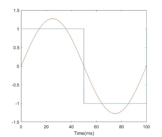
Let’s first look at a simple repeating square wave with a 50% duty cycle (ie half the time it is at high voltage, half the time it is at low. Fig. 26 shows a single pulse of a square wave with a pulse width equal to 10ms (5ms high, 5ms low). If we overlay a sinusoid with the same period as the square wave, we see that they have a similar shape, and indeed this sinusoid would be the first series of a Fourier series of the square wave, as we had previously illustrated in Fig. 11. Indeed, if we perform an FFT on the square wave, we will see the majority of the energy lies at this same frequency, as illustrated in Fig. 27.
|
Fig 26. Comparing a square wave with a sinusoid of the same period. |
Fig 27. FFT of the square wave waveform. |
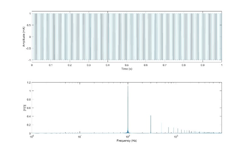
In this example the pulse frequency (100 Hz) is equal to the inverse of the pulse period since the pulses are sequential. Let’s take a look at what happens when we space out the pulses to create a pulse train with a pulse rate of a different frequency. In Fig. 28 we have a pulse train of pulses with the same amplitude and period as in Fig. 26, but with the pulses presented every 100ms (pulse frequency = 10Hz). We see that the power spectrum is more complex and spread out, however the majority of the energy is still centered around close to 100Hz (shifted somewhat to the left). There is some representation at the pulse frequency, but it is a small fraction of the total energy; we see that the pulse shape is far more important than the pulse frequency.
Fig 28. 10ms bipolar pulses presented at 10Hz.
Let’s add another variation to the pulses. One of the most common variations used is to introduce an interphase gap (IPG), which involves separating the positive and negative phases of the bipolar pulse. Let’s take the same 10ms pulses presented at that we examined in the last example, and insert a 10ms IPG, illustrated in Fig. 29. I’ve also inserted a sinusoid with a period of 30ms for comparison (the distance between the peaks of the sinusoid is equal to half the width of the two phases, plus the IPG; doubling this gives the length of the full period). If we now look at the pulse train made up of these pulses and calculate the FFT (Fig. 30), we see that the majority of the energy is spread around two centers; one at the frequency determined by the pulse width itself, but now there is more energy at the frequency determined by the pulse width and IPG. More energy is at the pulse frequency than compared to the last example, but it is still a minor component.
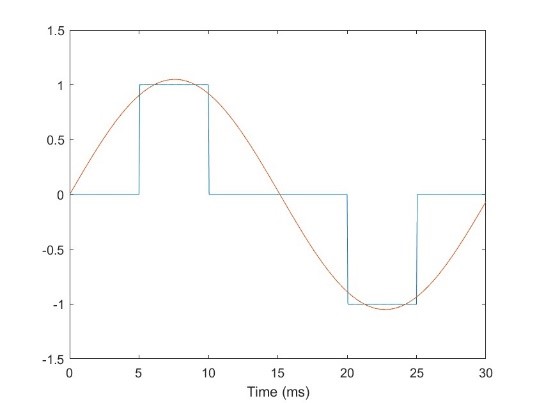
Fig 29. A bipolar pulse made of 5ms phases, with a 10ms IPG. A 33. Hz sinusoid is overlaid for comparison.
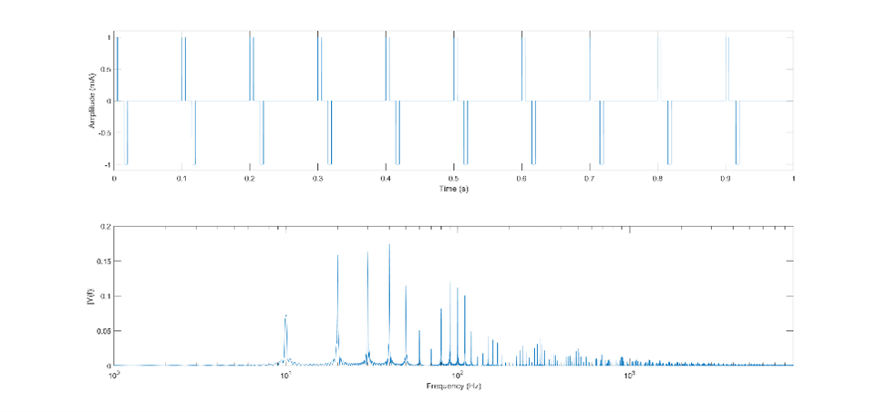
Fig 30. FFT of the pulse train made up of the pulses from fig. 25, presented at 10Hz.
Using the impedance curve illustrated in fig. 16 as a reference, in all of these examples we can see that if we were to either use the default 1kHz impedance measurement, or our pulse frequency to determine our how much current we could deliver, we would have been off by an order of magnitude, while using our pulse width provides us with a much more reliable figure.
If this still sounds complicated (and it is), the good news is that most stimulators have a voltage or current monitor so that you can test your stimulation protocol beforehand, as well as to monitor it on-the-fly during in vivo experiments. In general, voltage monitors are more useful for monitoring if the output is approaching the while voltage limit, while the current monitor is more useful for seeing if the output is approaching the current limit, but it is also more useful for verifying the shape of your intended waveform is being maintained. Since your electrode and subject provide a highly capacitive load, the voltage waveform can be highly distorted compared to the current, particularly with non-linear waveforms.
Fortunately, the PlexStim stimulator features both voltage and current monitors. To prevent artificial artifacts that can be created that can be created by a digitizing circuit, as well as report actual artifacts that can be missed by a digitized signal, the output of both monitors is driven by a purely analog circuitry, which can be connected to an oscilloscope for accurate representation (see fig. 31). Fig. 32 shows the output of both the current monitor (left) and voltage monitor (right) while outputting bipolar pulses with an IPG. Notice the oscillations at the corners of the square waves in the current monitor; these are called Gibbs phenomenon, or more colloquially as “ringing”. This will be present in all stimulators, although a digitized monitor is less likely to record them due to nyquist limitations. Also note how much the shape of the waveform in the output of the voltage monitor differs compared to the current monitor due to the reactive load. We can see that the voltage starts off at below zero while the current is being held at zero; this is because the tissue is negatively charged from the negative phase of the previous pulse, and so without a negative holding voltage current would flow back into the stimulator (and therefore have a nonzero current through the tissue). Likewise, there is a positive holding voltage during the interphase gap to prevent the positive charge from the positive phase from flowing back into the stimulator. During the phases themselves, the voltage starts out low and then increases in magnitude to match the rising charge in the tissue and maintain a constant current (the rate of this increase, or ramp rate, required to maintain the intended current will be proportional to the time constant, τ, of your electrode/subject load that we discussed early in the article).
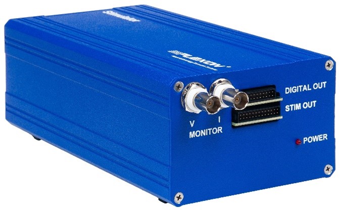
Fig 31. The PlexStim electrical stimulator has BNC output ports for both voltage and current monitoring. These outputs can be connected to an oscilloscope for high-resolution, real-time monitoring.

Fig 32. Output of the current monitor (left) and voltage monitor (right) of the PlexStim electrical stimulator while producing bipolar pulses with an interphase gap. The voltage output will vary considerably from the intended waveform due to the reactive load.
Effect on electroplated electrodes
As mentioned previously, electrodes sites are commonly coated with various materials such as PEDOT or platinum black to reduce impedance and/or make the sites less reactive and the impedance more stable over time. These coatings are generally applied through electroplating; in the process the electrode is immersed in a liquid a solution with a high concentration of the coating material, and a current is passed through the electrode sites and solution to draw the dissolved coating material to site locations, and held for an amount of time until the desired coating thickness is achieved. However even when not immersed in an electroplating solution, passing current through a coated electrode will cause movement of the coating material. This can lead to the material moving to the solution, ie your saline or subject’s interstitial fluid, leading to material loss over time. This can also lead to the material migrating to the center of the electrode site where the current density is highest, leading to dramatic increases in electrode impedance.
For these reasons, when stimulating it is best to use dedicated stimulation sites that are not electroplated. If this is not possible (ie you need to stimulate and record on all channels), then it is best to use an electrode with uncoated sites. If that too is not possible, then you should try to use stimulation parameters that are lower than the current used for electroplating, both in amplitude and for the amount of time used. For example, U, V and S probes are usually electroplated with PEDOT, and it is recommended not to exceed 30-60 μA of current, or a length of time of 2-3 seconds (notice the two ranges; going lower on one will allow you to go higher on the other without rapid damage). If you are unsure of the stimulation guidelines of your electrode, then it is best to check with the manufacturer or reseller.
Charge balancing and charge density
If an excess of charge builds up in brain tissue, it will interfere with cellular function in a number of ways, and lead to localized cell death. This is effect is taken advantage of intentionally during electrolytic lesioning, which can be used to mark electrode site locations following an experiment to make them visible during histological examination of the tissue, or during behavioral and cognitive studies to knock out brain regions to see the effect their absence has on behavioral or neural function. This is usually done with a low-amplitude, constant current over a long period of time (too high of an amplitude leads to significant heating, which can easily damage a larger region than is intended), or by using a slow switching current. Since, as mentioned early in this article, current is measured as movement of charge over time (one ampere is equal to one coulomb per second), if net current is allowed to move in one direction over a long of a period of time, it will lead to a build-up of charge that will be lethal to the affected tissue. Unfortunately this means that you can accidentally lesion the tissue that is the target of stimulation if care is not taken. If your stimulation waveform is not charge balanced it will inevitably lead to a buildup of charge, and therefore cause tissue damage during longer stimulating sessions. Likewise, if your stimulation waveform has too much amplitude for too long during a single phase of the stimulus, you can also deliver too much charge and damage your tissue. Let’s first examine charge balancing, and then we will explore how to determine the limits of amplitude and phase width of a charge balanced waveform to be safe.
In any bipolar waveform, the leading phase will charge the surrounding tissue (either positively or negatively), and the following phase will remove charge. If the area under the curve of the two phases do not match, then every pulse or period will add net charge to the tissue, eventually resulting in a lethal charge density and cell death. Waveforms that are symmetrical around the x-axis will automatically be charge balanced. Fig. 33 shows some charge-balanced waveforms with the charging phase highlighted in red and the discharging phase in green.

Fig 33. Waveforms that are symmetrical about the x-axis will always be charged balanced. The leading phase will charge the tissue, while the lagging phase will remove it.
However, as long as the areas above and below the axis are equal, charge will be balanced. Figure 34 shows asynchronous and biphasic and triphasic pulses. In both cases the amount of charge inserted into the tissue equals the charge that is drawn out by making sure that the amplitude times the duration of the total positive phases matches that of the negative phases. In the case of the triphasic, the tissue begins charging again mid-phase, but the charge is balanced again at the end of the third phase.

Fig 34. As long as the area of the positive and negative phases of a waveform are equal, the stimulation will be charge balanced.
However, even with a fully balanced waveform, if the duration and amplitude of a single phase is too high, it will create too high of a charge density and damage the tissue. Exactly how much charge is too much is tricky to quantify, and that is because the charge that is injected into the tissue doesn’t stay still, but will dissipate into surrounding tissue, and the rate of dissipation is hard to predict, and can vary greatly for a number of reasons. For instance, grey matter dissipates charge much more quickly than white matter; nearby blood vessels and bodies of CSF can very quickly shunt charge away. Even the subject’s current hydration level can significantly affect how quickly charge dissipates. As a result, attempts to quantify safe levels of charge density are a grey area, and are based on observational data with simplified factors. The most significant simplification is that rather than trying to quantify charge density as charge over volume since that is impossible to measure, as the charge will actually extend as a varying gradient throughout the subject and beyond. So instead protocols attempting to quantify safe levels of stimulation instead use charge over area, with the area being surface area of the stimulating electrode. This is usually measured a microcoulombs or nanocoulombs per square centimeter or millimeter (ie μC/mm2), but sometimes includes ph-1 (ie μC/(mm2*ph) or μC*mm-2*ph-1), where ph stands for phase, to stress that the measurement is across a single phase of the stimulus before the next phase subtracts from the charge.
When gauging the safety of cortical stimulator, the FDA will rate the stimulation as “safe” if it delivers less than 50 μC/cm2 per phase, “risky” if it is between 50 to 150 μC/cm2, and “dangerous” at levels above 150 μC/cm2. This criteria does not account the number of electrodes being stimulated through at once, and it makes no distinction between electrodes of very large areas vs very small. The latter is not surprising since the only FDA approved microelectrode array on the market is the Utah array; the vast majority of cortical electrodes are ECoG or sEEG electrodes, so this protocol is obviously designed with these electrodes in mind. An attempt at a more comprehensive guide is the Shannon equation, which used a large dataset of stimulation using electrodes of various sized and came up with the equation log(D) = k – log(Q), where D is the charge density in μC/cm2 per phase, Q is the charge in μC per phase and k is a value between 1.5 and 2.0, where from the dataset a k >= 2.0 always showed damage and a k<=1.5 damage was never observed (R. V. Shannon, A Model of Safe Levels for Electrical Stimulation. IEEE Trans. Biomed. Eng., vol. 39, no. 4, pp. 424–426, Apr. 1992.), similar to the “safe” and “dangerous” thresholds in the FDA guideline. Shannon recommended using a k of less than 1.5 for safety’s sake, however there have been reports that this can result in a stimulation level too low to elicit a response. If available, using a stimulation level that has been tested with the same or similar electrodes to those you are using, and has been shown to safely elicit the desired response, is ideal.
Whatever guideline you use, by taking advantage of the definition of an ampere as equal to a coulomb per second, ie ![]() charge per phase can be calculated by calculating the area under the curve for a single phase. For most non-linear stimuli this can be calculated geometrically; ie for square pulses simply multiplying the pulse amplitude by the pulse width, or for triangle or sawtooth waves multiplying one-half the amplitude by the phase width. For continuous waveforms, a simple integral over the first phase of the waveform can be calculated, ie
charge per phase can be calculated by calculating the area under the curve for a single phase. For most non-linear stimuli this can be calculated geometrically; ie for square pulses simply multiplying the pulse amplitude by the pulse width, or for triangle or sawtooth waves multiplying one-half the amplitude by the phase width. For continuous waveforms, a simple integral over the first phase of the waveform can be calculated, ie ![]() , where tps is the start of the phase, and tpe is the end of the phase. For instance, for a sinusoid that would be
, where tps is the start of the phase, and tpe is the end of the phase. For instance, for a sinusoid that would be ![]() , where A is the amplitude in amps, and f is the frequenty in Hertz. Solving this integral gives us Q = A/πf.
, where A is the amplitude in amps, and f is the frequenty in Hertz. Solving this integral gives us Q = A/πf.
Electrical stimulation and power dissipation
Another factor to be aware of is the total amount of power you are dissipating in your subject and electrodes. Power, measured in watts(W), is equal to IV, I2R or V2/R. One watt will heat roughly a quarter gram of water one degree Celsius every second; while that may not sound like a lot, even milliwatts can quickly cause severe burns if dissipated directly in tissue. Since P=I2R, higher levels of current in higher impedance electrodes can dissipate enough energy to damage tissue and electrodes. I have been approached several times by people who have wanted to stimulate on the order of a mA through multichannel silicon electrodes. Let’s use a smaller 16 channel electrode as an example, with impedance of roughly 1MΩ per site; that would be dissipating a peak wattage of 1W per site, totaling 16W in the electrode and subject. Sustained stimulation would literally cook a mouse, and would likely cause lethal damage to even a primate!
Thankfully with such high resistance, most stimulators would clip far below that level and not deliver anywhere near that amount of power (although as I mentioned previously, some clinical stimulators have compliance voltages of 100V or more, and so can easily deliver very dangerous amounts of power). However, even with a standard compliance voltage of around 10V, with a standard current limit of 1mA per channel, you can still output up to around 10mW per channel. That alone can be dangerous, and quickly adds up if stimulating across multiple channels.
Even at sub-lethal amounts of power, it is also important to be aware that even small amounts of tissue heating can significantly change the electrophysiological behavior of neural tissue, possibly creating a confound in the results of your study. Therefore it is a good idea to take the time to make an estimate of how much power you will be delivering to your subject, particularly if stimulating across a large number of channels, stimulating with rapid or wide pulses, high amplitudes, and/or are delivering sustained stimulation.
Summary and take-aways
- Single unit quality is mostly determined by the surface area of recording sites. While electrode impedance is related to the electrode diameter, it is also greatly impacted by electrode material, treatments and coatings. So, while impedance can be a good predictor of unit quality between electrode sites of the same array, or between electrodes of identical design, or the condition of an electrode over time, it is not useful in comparing between electrodes of different materials and designs.
- Electrodes with excessively high impedance (compared to the input impedance of the headstage) will suffer from low signal-to-noise, making it difficult to impossible to record spikes.
- Monitoring electrode impedance over time is very helpful both in trouble-shooting recordings and maintaining the longevity of your probes.
- If electrically stimulating, care should be taken not to exceed the compliance voltage of your stimulator to ensure you are delivering the correct amount of current. The varying impedance of electrodes in respect to frequency, and the wide frequency spectrum of nonlinear stimulation patterns can make this difficult. When in doubt, using a stimulator’s voltage and/or current monitor feature to verify.
- Care should be taken when electrically stimulating through electrodes with coated recording sites to avoid damaging them.
- Care should be taken during electrical stimulation to avoid accidentally lesioning tissue through excess charge.
- Care should be taken not to deliver too much total power when electrically stimulating if stimulating across a large number of channels, stimulating with rapid or wide pulses, high amplitudes, and/or delivering sustained stimulation.
Links to references and further reading
Wikipedia page on Complex Numbers
Causes of Noise in Electrophysiological Recordings, Plexon blog post June 28th, 2021
Wikipedia page on Fourier Series
Wikipedia page on Fourier Transforms