Electrodes, as the name implies, are electrical devices, even if passive ones, and therefore their performance is affected in several ways by electrical impedance. How their performance is affected is commonly misunderstood, in particular there is a common misconception that higher electrical impedance means greater isolation of single units, and lower impedance electrodes will result in poor or no units. While there is a relationship between unit quality and impedance, it is not as simple as high impedance is good and low impedance is bad. In this article we will look at how electrical impedance affects recording quality by first looking at what impedance is, and then use that understanding to explore how it affects the electrophysiological signal.
Electrical Impedance, What It Is and Types of Impedance
Impedance, measured in ohms, is the measure of how rapidly charge will flow through a material due to an electrical potential. The flow of charge, called current, is measured in Amperes (or amps for short); one ampere is equal to one coulomb of charge flowing per second. Electrical potentials are measured in volts (a one volt potential is fundamentally defined as the field that will add one electronvolt of kinetic energy to an electron that passes through it; it can also be defined by its relationship to current and impedance as we will soon see).
There are two types of impedance, resistance and reactance. Simple resistance does not change with the frequency of the signal, whereas reactance does. Since we are looking at signals that vary with time (ie action potentials, local field potentials) it is reactance that is going to have the most impact on our recordings, however since simple resistance is much easier to explain, we are going to start with that.
Examining the Relationship of Resistance, Current and Potential Using the Hydraulic Model
Ohm’s law states that V = IR, or alternatively I = V/R or R = V/I, where R is the resistance, V is the potential (or voltage after its unit of measurement), and I is the current (I is still used as it was in André-Marie Ampère’s famous 1882 paper to denote “intensité de courant”). Using the Ohm’s law we can see that if we pass a 1A (ampere) current through a 1Ω (ohm) resistor, it will create a 1V (volt) potential across the resistor. Alternatively a 1V potential will create a 1A current if applied across a 1Ω resistor, or if you measure 1A of current passing through a resistor, and measure a 1V potential across it, you know it’s impedance is 1Ω. From this we can see that current is proportional to voltage with a fixed resistance, or inversely proportional to resistance with a fixed voltage.
This relationship can be more intuitively understood by using what is called the hydraulic model; imagine a cylinder of water with a hose at the bottom (Fig. 1). Filling the cylinder with water will create water pressure at the opening of the hose; the higher you fill the cylinder the more pressure it will create. You can think of the pressure as potential. Water will flow out of the end of the hose, how much water flows (ie in milliliters per second) can be though of as current (coulombs per second). How much water the hose slows down the flow of water can be thought of is the resistance; ie a wider diameter hose will have less resistance to the flow of water compared to a thinner one (shortly we will examine the relationship between resistance and cross-sectional area of a conductive medium). Filling the cylinder to a higher level will increase the flow of water (increasing V in I=V/R) as will using a fatter hose (decreasing R in I=V/R).
Fig 1 hydraulic model
This model would work well if all conductive materials had the same amount of resistance in relation to their volume and length, but that is not the case. Therefore a way to improve the model would be to think of the hose as filled with a porous material, such as finely packed sand or loosely packed cotton. This is a good way of thinking about it, since in a solid conductive material the charge carriers (electrons) flow through the matter around the nuclei, with the interactions between the charge carriers themselves and the nuclei causing resistance (called electron-phonon interactions). This is similar to the resistance that water sees flowing through a porous substance, where the resistance to flow is caused by the water itself (since water has volume) as well as the solid part of the material.
With the resistive material it becomes obvious that the longer the water has to travel through the resistive material the more restricted the flow will be, ie with a hose of packed sand you can expect the flow to double if you cut the hose in half. So now we have three ways that we can reduce resistance; we can still increase the diameter of the hose, decrease the length of the hose, or use a more porous material inside the hose (see Fig. 2).
Fig 2 hydraulic model with porous material
We can calculate the resistance of a piece of conductive material if we know its dimensions and its electrical resistivity, ρ, commonly measured in Ω·m or Ω·mm (ohm meters or ohm millimeters). ρ can vary significantly between materials; ρ of silver, the most conductive elemental metal, is 15.87 nΩ⋅m, whereas for pure silicon it is 2.3 kΩ⋅m, more than 11 orders of magnitude difference (I should point out that silicon electrodes are not pure silicon. Pure silicon is a semiconductor and would not provide a usable signal; instead it is doped to act as a conductor, although it is still significantly more resistive than metals). The relationship between resistance and resistivity is , where l is the length of the material and A is the cross sectional area (see Fig. 3).
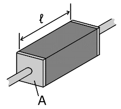
Fig 3. The resistance of an individual conductive element is a function of it’s resistivity, length, and cross-sectional area. Image from Wikipedia.
Let’s use the formula to calculate a sample impedance; let’s say for a 10mm long piece of cylindrical platinum wire, with a 15um diameter, insulated on the sides. Platinum is a metal commonly used for electrodes both for its stiffness (less likely to deform during implantation) and inertness (which increases its biocompatibility). Actually, platinum electrodes are usually a Platinum-Iridium alloy (pure platinum is much softer), but as an alloy the electrical properties can vary with alloy proportions, so for simplicity we’ll stick with pure platinum in this example, which as you’ll soon see won’t have a significant effect on the results. Platinum has an electrical resistivity of 105 nΩ⋅m, so a 10mm long platinum electrode with a diameter of 15μm (or radius of 7.5μm), insulated on the sides, would have a resistance of:

And this is what you would measure if you connected an ohm meter directly to the electrode. However that is not the way we measure impedance, not because it is difficult, but because the measurement wouldn’t be very useful. Instead we immerse the electrode in saline as this gives us results much closer to an electrode in tissue, and if you have ever measured the impedance of a platinum electrode (or just about electrode designed for electrophysiology) in saline or in vivo you have likely found that the impedance is many magnitudes of order higher; on the order of tens of kiloohms (1kΩ = Ω ) to megaohms (1MΩ = Ω). Obviously since the current has to pass through the saline to reach the electrode, the resistance of the saline will have an effect. However we know the resistivity of saline (although it varies with salinity, ie how much salt is dissolved in the water), and although it is many orders of magnitude higher than metal (about in salinities close to cerebrospinal fluid or CSF), the cross-sectional area is much larger (the diameter of your beaker is measured in cm rather than μm), if we were to use the above formula to calculate the resistance of a beaker of saline it would also be on the order of ohms. So obviously something else is going on here, and what that is is that whenever you put a solid conductor into an electrolyte, you get what is known as an electrolytic capacitor. Capacitance is one of the main components of reactive impedance (the other being inductance, however inductance has far less impact that capacitance in electrophysiological recordings so we will not discuss it in this article), so let’s examine capacitance and how it affects impedance.
What is Capacitance?
The Parallel Plate Capacitor
Capacitance is the ability of an object to store charge. It is measured in farads (F), named after Michael Faraday, whom the Faraday cage, another useful tool for electrophysiologists, is also named after. Capacitance is defined as C = q/V, where C is the capacitance, q is the charge, and V the potential or voltage. As you can see from the formula, at a fixed voltage, the larger the capacitor the larger the amount of charge it can hold. A one farad capacitor can hold one Coulomb of charge when allowed to fully charge from one volt. Although one volt is a small potential, one coulomb of charge is huge; allowed to quickly dissipate into a human body it would easily kill that person. One farad is also a huge amount of capacitance; usually the size of a large coffee can you, will not likely encounter a 1F capacitor outside of a power station, so the units μF, nF and pF are more commonly used (a picofarad is farads). Since capacitors hold charge, and current is the flow of charge, and impedance is the resistance to flow of charge, it should be easy to see that capacitance will have a large effect on impedance.
The simplest form of a capacitor is a parallel plate capacitor; as the name implies it is made up of two parallel plates of conductive material with a dielectric in between. It is the inspiration for the schematic diagram symbol of a capacitor. A dielectric is an insulating material, ideally with high permittivity, ie it will not pass current but polarize more strongly in an electric field, allowing more charge to be held at either end (see Fig. 4). The capacitance of a parallel plate can be calculated using the formula C = , where ε is the permittivity of the dielectric, A is the area of the parallel plates, and d is the distance between the plates or thickness of the dielectric (see Fig. 5).
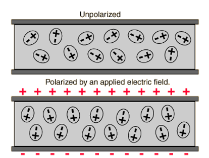
Fig 4. A material with higher permittivity is more easily polarized in an electric field, and able to hold more charge at its surface. Image from Wikipedia.

Fig 5. Structure of a parallel plate capacitor. Image from Wikipedia.
If a battery is connected to a capacitor (see Fig. 6), electrons will flow out of the negative terminal of the battery and start charging what is now the negative plate of the capacitor. Likewise electrons will flow from the positive plate into the positive terminal of the battery, both pulled by the positive charge of the positive terminal, and repelled by the negative charge building up on the negative plate. This will continue until the capacitor has the same voltage as the battery, at which point the capacitor is fully charged with a charge of q = CV and the current will stop. How long this takes is determined by both the size of the capacitor in farads, and the resistance of the entire system, or circuit (the battery, wires and capacitor itself will all have some small amount of resistance), so that τ = RC, where τ, called the time constant, is the amount of time it will take to charge the capacitor to about 63.2% of its capacity (63.2 ≈ 1-e-1). Likewise if the charged capacitor is then detached from the battery and attached to a new circuit of resistance Rn, τn will be the amount of time for the capacitor to discharge to about 36.8% of its capacity (36.8% ≈ e-1). Charging can be modeled as V(t) = Vo(1-e-t/τ) where V(t) is the voltage across the capacitor at any given time, and Vo is the initial voltage (zero if uncharged). Likewise discharging can be modeled as V(t) = Vo(e-t/τ). This time constant will have some interesting consequences when we start looking at what happens when we put an alternating voltage across the voltage.
Fig 6 capacitor charged by a battery
If we put a sinusoidally alternating voltage across the capacitor, the voltage source will alternate between which plate it is pushing charge into and which it is pulling it from. However whichever plate is being charged will be at a point of maximum charge when the sinusoid transitions, ie the sinusoid is at 0V between the positive and negative phase or vice versa (see Fig. 7), after which the voltage flips polarity and charge is moved to the opposite plate. Since that is the point of maximum charge, it is also the point of maximum repulsion from the charge on the negative plate. As a result, while a capacitor will stop current from flowing once it is charged from a direct voltage (at that point act as an open circuit, or infinitely resistive), an alternating voltage will pass, but will be phase shifted by some amount less than 90֯ (it would be exactly 90֯ if there were no resistance, but since that is physically impossible it will be some amount less; this will be equal to the phase of the complex impedance as described earlier).
Fig 7 capacitor charged by an alternating voltage
Using the hydraulic model we can more intuitively understand a capacitor as a flexible membrane across the inside of a sealed tube of water. Exerting a constant pressure of water on the membrane will cause it to stretch; the greater the pressure the greater the membrane will stretch and the greater the volume of water the stretched cavity will hold (equivalent to the amount of charge). A more flexible membrane (higher capacitance) will stretch further at the same amount of pressure, but regardless will eventually stop the flow of water. If the pressure is removed, the membrane will spring back and create a flow of water in the opposite direction, just as a capacitor will relinquish its stored energy by giving back the charge it held. If you were to apply an alternating pressure, a stiffer membrane (lower capacitance) will translate less of the alternating pressure to the other side, creating more resistance to the movement of water. Electrical capacitors work the same way, and their impedance at a given frequency is inversely proportional to their capacitance. Just as a capacitor is an open circuit to a direct voltage, its impedance also drops off with higher frequency. The impedance of a capacitor can be calculated as Z = , where C is the capacitance and is the frequency of the driving voltage or current. Notice that impedance is commonly denoted as a “Z” to indicate that it is a complex number, including both real (resistance) and imaginary (reactance) components. The j is to indicate that it is an imaginary number equal to (mathematicians more intuitively use i for imaginary numbers, but engineers generally use j to avoid confusion with current). Complex numbers are a topic that are too complex for the scope of this article (although wikipedia has an excellent explanation), it is enough for our purposes to know that normal numbers are scalars, having only magnitude, whereas complex numbers are vectors, having both magnitude and direction, or phase. The magnitude of a complex number can be calculated using Pythagorean’s theorem, and the phase with trigonomic functions (ie for a 1Ω resistor in series with a 1F capacitor driven by alternating voltage with a frequency of 1/2πHz to give -1Ω of reactance, the magnitude of the impedance would be , resulting in a current of (1/)A phase shifted 45֯ relative to the voltage). Therefore, an impedance containing reactance will not only attenuate a signal, like a purely resistive impedance will, but also cause a phase shift. This will cause some interesting effects on a complex signal that is made up of more than simple sinusoids, as we will see later.
The Electrolytic Capacitor

So now let’s look at why a solid conductor in electrolyte acts as a conductor. You may be surprised to learn this, but pure water is actually an insulator. When two hydrogen atoms bind to oxygen, the electrons will sit deep in the electrostatic potential of the oxygen nucleus. This creates a highly electronegative atom, with a strong positive charge on the side of the molecule with the hydrogen nuclei (protons), and a strong negative charge on the side with the oxygen nucleus. Because of this high level of electronegativity electrons cannot flow across the molecule, but it also makes water a very strong polar solvent, capable of dissolving compounds such as salts since it will rip positive and negative ions away from each other (it is because of this strong electronegativity that such water is liquid instead of a gas at STP despite being made up of such light-weight molecules). With water full of anions (negative ions) and cations (positive ions), the ions can now freely flow, moving charge, and making water conductive. This is why you wouldn’t want to jump into a vat of purified water holding a plugged-in toaster; although initially the water wouldn’t conduct, the salts on the surface of your skin would immediately dissolve and the water would now have charge carriers available to give you a strong jolt. The more ions dissolved in the water the more conductive it is, so dissolving sodium chloride in water to match the molarity of dissolved ions in cerebrospinal fluid or the interstitial fluid of the brain and nerves will make a good model to test the impedance of your electrodes.
Fig 8 pure water vs saline
The action potentials created by excited neurons are the result of the neuron controlling the flow of ions through ion channels, particularly sodium and potassium, but also calcium, chlorine, magnesium, etc. These ions can travel freely in solution, but cannot travel through a solid conductor. If a potential is created it will cause anions or cations to travel to the surface of the electrode, but they cannot penetrate the electrode to create a current the way that electrons can flow through solid conductors. Instead a flow of anions like chlorine toward the surface of the electrode will repel electrons away from the surface of the electrode, just the way that a flow of electrons into one plate of a parallel plate capacitor will cause electrons to be driven away from the plate/dielectric junction at the opposite plate. Similarly cations like potassium and sodium flowing towards an electrode will attract electrons to the surface of the electrode, just like a positive charge on one plate of a parallel plate capacitor drains it of electrons, creating a net positive charge that attracts electrons towards the opposite plate/dielectric junction. It is these flows of charge carriers that can move freely within their medium, but not cross the solid conductor/electrolyte junction that creates a capacitive effect.
Fig 9 electrolytic capacitor junction
Industrial electrolytic capacitors will oxidize the surface of the metal before placing it in electrolyte; this creates an easily definable dielectric layer that makes the capacitance easy to calculate, and therefore easy to design the dimensions needed for a specific capacitance value. Since an electrode in electrolyte does not have this clearly defined layer, capacitance is not easily predicted or calculated, however the capacitance of platinum in saline has been experimentally measured to be approximately 0.2pF/ (DA Robinson, The Electrical Properties of Metal Microelectrodes. Proceedings of the IEEE, Vol 56, No 6, June 1968). If we use this value for our 15um diameter platinum electrode that we looked at earlier in the article, and a frequency of 1kHz (we will explain in the next section why we are using 1kHz), this a capacitance of π*(7.5, which gives us a magnitude of impedance of |Z| = ≈ 4.5MΩ. Although this is actually about two orders of magnitude above what you would measure from a 15μm diameter platinum wire, we can see we are now getting into the ballpark. There are a few reasons for the difference (all of which are discussed in the Robinson paper if you would like more details), but the most significant is that an electrolytic capacitor actually has a leakage resistance in parallel with the capacitive load (see Fig 10, we will discuss later what loads in parallel and in series means, but for now know that any number of loads in parallel always have less total impedance than any individual load). This leakage resistance is created because cations and anions in solution can accept or give up electrons, and in turn transfer them to or from the solid conductor, creating a leakage current, hence the name.
Fig 10. Equivalent circuit model of an electrolytic Capacitor. Note that while the resistors noted represent simple resistance, they are being represented by the symbol more commonly used for a complex load consisting of resistance and reactance (ie a rectangle instead of a squiggle). This is to denote that these values are frequency-dependant. The symbol for LESL denotes inductance, which as previously mentioned is not explored in this article, and does not significantly contribute to the total impedance in the frequency ranges of interest to the electrophysiologiest. Figure from Wikipedia.
We won’t repeat this calculation for a silicon electrode as there are too many variables (the level of doping will significantly all of the values discussed), but the higher resistivity of the material will result in a lower capacitive value along with a lower leakage current, resulting in much higher total impedance. In general silicon electrodes have an impedance of around two orders of magnitude higher than a metal electrode with the same site diameter recording sites. However these values can also be changed significantly by doing things such as abrasive treatment of the electrode sites (this increases the surface area without increasing diameter, which in turn increases capacitance and leakage current, reducing impedance), or coating the recording sites with different conductive materials such as platinum black or PEDOT, which will also significantly affect capacitance and resistance, and therefore impedance.
Complex Signals and Frequency
So far we’ve been calculating our impedances in relation to a pure sinusoid voltage of 1kHz; this (or a frequencies close to it) is the default frequency generally used by most impedance measurement devices (such as the nanoZ or IMP, although they are capable of measuring at different frequencies) and by electrophysiologist in general. Lets take a look at why that is.
Any biological signal is unlikely to be a pure sinusoid, however any signal can be constructed by summing up an infinite series of sinusoids, known as a Fourier series (as illustrated below in Fig. 11). Likewise a Fourier transformation can be performed on a signal or function to show the power spectrum of a signal, ie where the energy of the signal lies in relationship to frequency (see Fig. 12). If you were to perform a Fourier transformation on a signal, then use that spectrum to calculate the effects of your complex impedance, by transforming those results back into the time-amplitude domain (ie perform an inverse Fourier transformation), you can calculate how any signal would be affected by a complex impedance. The mathematics of a Fourier series and Fourier transform are beyond the scope of this article (although if you’d like to learn more, the wikipedia pages are very informative, or you could look at just about any textbook on signal processing), but having an awareness of these concepts will help understand why frequency is important to electrophysiology.
| Fig 11. A square wave being approximated by the sum of the first four terms of its Fourier series. Animation from Wikipedia. | Fig 12. The relation of a signal, its Fourier series (using the first 6 terms), and its Fourier transform/power spectrum. Animation from Wikipedia
|
In this article we will use the Fast Fourier Transform (called FFT for short) on various signals to illustrate the effects of frequency. The FFT is an approximation of the Fourier transformation that can be done on a digitized signal with a digital processer. Fig. 13 shows a 10Hz sinusoid plotted in the time domain on the top, and frequency domain on the bottom using an FFT calculated in MATLAB. A Fourier transform would simply be a vertical line at 10Hz, with an amplitude of 1, and zero elsewhere, but the FFT approximation is more than close enough to be useful for our purposes. Likewise Fig. 14 shows approximated white noise (generated using MATLAB’s rand function). A Fourier transformation of true white noise would be a horizontal line. The FFT shows the limitations both of an FFT of a limited sample size and in digitally generating signals; it is limited in the higher frequencies to half the sampling rate (called the Nyquist frequency), and the power isn’t accurately measured in the lower frequencies due to the short length of time of the signal. In both cases the FFT would more closely resemble the results of a Fourier transform with a larger sample set.
| Fig 13. A 10Hz sinusoid plotted in the time and frequency domains | Fig 14. Approximated white noise. |
Let’s now take a look at how an impedance meter works. Basically an impedance meter is a current source that feeds a current of known frequency and amplitude into a test load (in our case an electrode in saline, or for an in vivo test, and electrode inserted into a subject), and then records the resulting voltage across the test load (see Fig 14.). Using Ohm’s law for a complex impedance, Vload = Itest x Zload, we can measure the magnitude of the impedance of that load by comparing the amplitudes. By comparing the phase difference between the test current and resulting voltage, we can also calculate how much of the impedance is real (resistance) and how much is imaginary (reactance), and therefore measure the simple resistance and capacitance of the electrode. Pure sinusoids are used because they are easy to accurately produce with an oscillating circuit, easily measured, and since the mathematics are simpler, easier to accurately assess the results digitally. By varying the frequency of the test signal used, we can measure the impedance spectroscopy of the electrode, which is a curve of impedance vs. frequency (see Fig. 14 for an example impedance curve of an S-probe measured with the impedance spectroscopy feature of a nanoZ). If we know the frequency characteristics of the signal of interest, we can then use the impedance curve to predict how the electrode impedance characteristics will impact our recordings.
| Fig 13 impedance tester schematic Fig 13. … | Fig 14. Impedance spectograph of a 16 channel S-probe with 15μm diameter recording sites. Recorded with a nanoZ from 1.005Hz to 2kHz. Both axes are logarithmically scaled. Notice that the impedance drops from tens of megaohms in the hertz range to tens of kilohms in the kilohertz range. |
Since we are interested in recording single units, lets take a look at an action potential. Fig. 15 shows a pile plot of several action potentials from a single unit recorded on an Omniplex system, from an anesthetized mouse acutely implanted with a Michigan array. The units were thresholded and separated in Offline Sorter, and one unit selected and exported to Matlab for analysis. Overlaid on the pile plot is one cycle of a 1kHz sinusoid for comparison. As you can see from the comparison, the main body of the action potential is a little bit thinner than the cycle of the sinusoid, suggesting a center energy that’s a little higher than 1kHz. And indeed, if we look at the FFT we can see that the peak energy is close to, but a little higher than 1kHz. This will vary a little bit among different neurons and types of neuronal populations, however we can see that this is why we measure impedance at 1kHz (or near 1kHz), since that is the lion’s share of where the energy lies in single units, and where the signal will be most impacted.
| Fig 15. A pile plot of action potentials recorded from a single unit with a 1kHz sinusoid overlaid for comparison | Fig 16. FFT of the action potentials |
This of course assumes that your focus is single units. If you are more interested in local field potentials or electrocorticography, then you will want to pay more attention to the lower end of the frequency spectrum. However, we will soon see that there are several factors that make recording these signals much less challenging, and therefore do not usually require the same level of attention.